Customer Segmentation
Customer segmentation is the practice of dividing a customer base into groups of individuals that share similar characteristics, such as age, gender, interests, and spending habits. This process recognizes the uniqueness of each customer, enabling businesses to optimize their marketing strategies by delivering personalized messages to smaller, targeted groups. By gaining deeper insights into customer preferences and needs, companies can effectively tailor their marketing materials, resulting in enhanced value for each segment.
This tutorial aims to classify new clients into four distinct classes (A, B, C, and D) based on various client attributes, including age, gender, education status, profession, and more. The dataset used in this tutorial contains client information.
To accomplish this classification task, we will use the PapAI platform, specifically leveraging its multi-classification models. These models will enable us to identify shared characteristics among clients within each class accurately.
Create a project
Upon logging into papAI, you will be directed to your project homepage. This page showcases all the projects you have created or are collaborating on with other members. To initiate a new project, simply click on the New project button, which will open a pop-up window with various settings to complete. These settings include the project name, a brief description, the persistency setting, and the desired sampling technique. You can specify the number of samples to display and select the order, such as the first or last N rows or randomize the selection. Once you have filled in all the necessary settings, finalize the process by clicking on the Create button. Your new project will automatically be added to your main page, ready for you to begin working on. With papAI, starting a new project has never been easier!
Here is a video showing the project creation process on papAI
Import datasets
With papAI, you have the flexibility to import data from a wide range of sources, allowing for seamless analysis and visualization in your project. Whether you choose to import data from your local machine, external databases (SQL or NoSQL), cloud storage, or an API, papAI provides a straightforward process for data integration. Additionally, you can create entirely new datasets using the dedicated Python or SQL recipe editor, expanding your analytical capabilities even further.
Here is a video showcasing the data import process on papAI
To begin importing your data, you can utilize the tools available in the papAI interface. For our particular use case, we will import our dataset from our local machine. To access this tool, simply click on the plus button located in the top right corner of the interface, or you can utilize the Import dataset button in the Flow interface.
Here is a video of importing a dataset from a local machine
Once you select the local import option, a new interface will appear, allowing you to effortlessly import tabular files in either CSV or XLSX format. You have two options for importing your desired files: either click the Import button or utilize the drag-and-drop feature. After importing your data, you can preview a subset of it to ensure correct importation. Once you have confirmed everything is in order, proceed by selecting the Import button to initiate the uploading process. A progress bar will provide updates on the upload status, and once complete, your dataset will be readily available for use in your project's flow.
Visualizing and analyzing the dataset
Once you have imported your dataset into papAI, you can start exploring its content and conducting an initial analysis to identify the necessary cleaning steps required to extract valuable insights. However, before delving into preprocessing, it is crucial to examine the data's structure through data visualization.
To do this, simply double-click on the database, which will enable you to view the structure of your database.
Here is a video that shows how to visualize the content of the data
papAI simplifies the process of visualizing your data. To access the dedicated visualization module, double-click on the desired dataset and select the Visualization tab located in the top right-hand corner of the interface. From there, you can choose from various graph options and select the columns or aggregations to be represented and displayed in your chosen graph format. Some graphs additionally allow you to define a colormap for a legend and filter out specific values to focus on specific aspects of your data.
For a more comprehensive data analysis, you can use descriptive statistics to identify trends and gain a better understanding of the distribution of your data. In papAI, accessing these statistics is straightforward – just navigate to the Statistics tab within the table interface.
Here a video showing the generated statistics by papAI
This interface provides a convenient way to view important statistics for each column in your dataset, including the median, mean, and standard deviation. Additionally, you can visualize the distribution of your data using graphs like box plots and histograms, which offer a comprehensive understanding of its characteristics.
Analyzing these descriptive statistics enables you to gain valuable insights into your data, identifying any outliers or trends that may require further investigation. This information can guide your preprocessing and modeling choices, leading to more precise and dependable results.
Advanced Visualization
Here is a video of advanced visualization features
Through visualizing the segmentation of individuals based on their marital status, we observe that the majority of segments A, B, and C comprise married individuals. Conversely, segment D predominantly consists of non-married individuals.
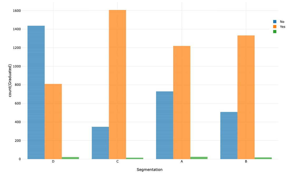
Through visualizing the segmentation of individuals based on their graduate status, we observe that the majority of segments A, B, and C consist of graduated individuals. On the other hand, segment D primarily comprises non-graduated individuals.
Hence, it can be inferred that there is a correlation between marital status and graduate status.
Here is a video of advanced visualization features
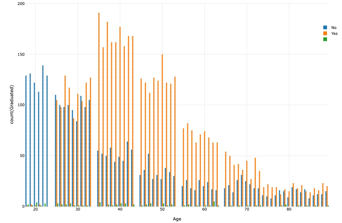
We have observed that individuals in their 20s and 30s mainly fall under segment D, while those in their 40s mainly fall under segment A. Finally, Most of the individuals in their 50s or older are in segment C.
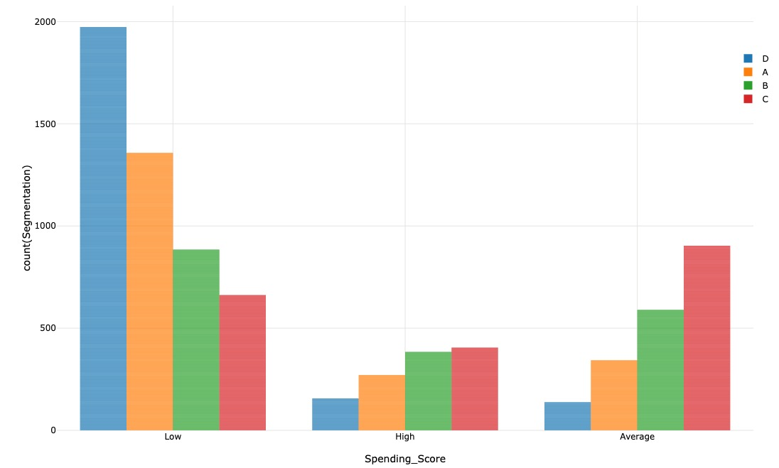
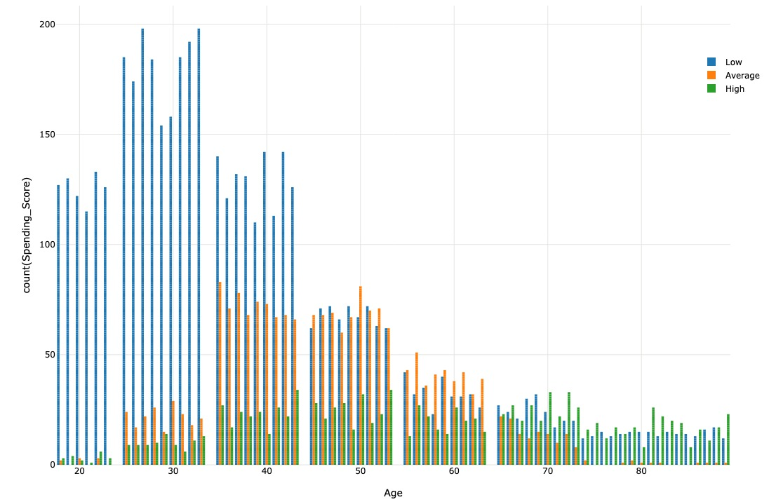
We noticed that individuals with a low spending score are primarily in the D segment, whereas those with an average or high spending score are usually in the A, B, or C segments. Furthermore, most of the individuals in the dataset had a low spending score.
Throughout the observations made, we can notice that segment D represents individuals with a low spending score. They are mainly not married, nor graduated, and are in their 20s or 30s. As they get older, their spending score tends to increase; many get married as well.
Data pre-processing
Here is a video of data pre-processing using PapAI
To train the model, we need to convert the data from categorical to numerical format. To do so, we can use PapAI's pre-processing features such as Change Cell and Cast Column.
Here is a video of data pre-processing using PapAI python Recipe
Since we will need to repeat this process for other columns, it is more efficient to use PapAI's Python Recipe.
Note
You can apply more complex operations through Python or SQL scripts if you are more familiar with these programming languages.
# read the dataset from flow
df = import_dataset("Train")

# change the values of columns and their type from string to int

df['Ever_Married']=df['Ever_Married'].replace({'Yes':1,'No':0})
df['Gender']=df['Gender'].replace({'Male':1,'Female':0})
df['Graduated']=df['Graduated'].replace({'Yes':1,'No':0})
df['Spending_Score']=df['Spending_Score'].replace({'Low':0,'Average':1,'High':2})
df['Profession']=df['Profession'].replace({'Homemaker':0,'Marketing':1,'Healthcare':2,'Artist':3,'Executive':4,'Lawyer':5,'Doctor':6,'Engineer':7,'Entertainment':8})
df['Var_1']=df['Var_1'].replace({'Cat_1':1,'Cat_2':2,'Cat_3':3,'Cat_4':4,'Cat_5':5,'Cat_6':6,'Cat_7':7})

# export a dataset to the flow
export_dataset(df, "df_process")
Train and test the model
At this stage, your dataset is ready to be used for training and testing models and choosing the right one to be deployed in production. To do this, we first split the dataset into two separate datasets: one for training and the other for testing. To do this, select the dataset and then click on the *** Split rows *** operation from the green icons in the left sidebar. A pop-up will appear which allows you to tune some settings such as the names of the two created datasets, the splitting order (in our case it will be 80/20%), and the splitting method. After setting all the preferences, click on the "Save and run" button to apply the split.
Here is a video showcasing the split operation applied to our dataset
After splitting and creating the training and testing sets, we can initiate the ML process by clicking on the training dataset and then the ML Lab icon. This will give us access to the ML Lab, where we can test various models. Before, however, we must define the use case we want to tackle. Crafting a ML use case is easy, as all we have to do is click on the 'New Use Case' button. This brings up a pop-up, allowing us to choose the kind of use case we need to address our issue; in this case, it is a multi-classification problem. In addition, we must fill in certain fields, such as the target which is the segmentation, (while also adding a transformer, if necessary). Finally, we simply need to name our use case and click on *** Create *** to gain access to the ML Lab and store our progress.
When accessing the ML Lab, you can easily create and build an ML pipeline from scratch, with multiple models and parameters to optimize the process and extract the best model without any coding. The first step is Feature selection where you select the features to be taken into account in the model training, and also apply some preprocessing to ensure better results.
Model selection is the next step where you can select regular ML models with their default parameters such as Logistic Regression, Random Forest and Decision Tree by toggling the button next to them. After that, you enter the Evaluation step where you modify the size of the validation set to 0.2, then launch the training process by clicking the Train button. The progress of each run is stored in a table, allowing you to follow the performance of each model.
Here is a video showcasing the training of the ML models chosen
Evaluate and Interpret the model
The evaluation of each model is essential, as one of them will be used to predict customer segments. Our prediction must be accurate and avoid any errors that could result in serious issues. With the ML Explainability module, we can display tools and graphs that accurately describe the model's decision-making process for the prediction, making it easier to understand the underlying mechanism of the algorithm. To access this module, simply select a run from the list of runs in your use case.
Here is a video showcasing the evaluation of the ML models chosen
You will have access to the XAI (Explainable Artificial Intelligence) module related to the trained model you chose. The first part of this module is evaluation, where you can assess the model's performance through metrics such as accuracy, precision, recall, and ROC AUC score. You can also view visualizations such as a confusion matrix and ROC curve - these are essential for judging the model's efficacy. The second aspect focusses on the underlying mechanisms of the model - specifically how the features affected the decision-making process during training. This is displayed by the Feature Impact and Tree Surrogate tools. The Feature Impact tool classifies each feature by its influence over the model's predictions, and shows the target probability varying with the value of one feature. The Tree Surrogate tool displays the leaves created by the model, providing useful insights about its decision-making process.
Test the predictions made by the model
Coming to the final step of this tutorial, you have chosen the right model to deploy it for your case, but you still need to test it on the testing sample you created earlier to get accurate predictions. To resolve this issue, you need to add the newly trained model into a model registry by identifying the model run, checking the box next to it and selecting the Add to Flow action from the Actions list at the top of the ML Runs list. This will trigger a small pop-up window to set up the model registry and fill in some fields such as the registry name, the recipe name, and the activation method. When done, you simply hit the "Create" button, and the model registry will be created and displayed on your Flow.
Here is a video showing the model registry creation process
Creating a model registry will allow you to calculate any prediction on a chosen dataset. To initiate the prediction process, select the dataset and select the Prediction option on the left sidebar. Choose the registry you wish to use and click Continue. A small pop-up may appear offering optional settings that you can adjust if necessary. When complete, click the Save & Run button to activate the prediction process, creating a new dataset with a column displaying the predictions of the target class.
Here is a video showcasing the prediction step triggered
In conclusion, by following these simple steps, you can easily complete your data science project from start to finish without any coding knowledge. We hope this guide was helpful to you. If you want to learn more, please check out the extensive collection of tutorials offered in the papAI library, which will provide more detail on additional features and capabilities.